Neural networks 101
The purpose of this article is to serve as an introduction to understand what Neural Networks are and how they work, without all the heavy math.
If you want something more advanced with fancy equations and what not, you should check the links at the end of the article.
So, let's start from the basics
Neuron
Neurons are the basic unit of a neural network. In nature, neurons have a number of dendrites (inputs), a cell nucleus (processor) and an axon (output). When the neuron activates, it accumulates all its incoming inputs, and if it goes over a certain threshold it fires a signal thru the axon.. sort of. The important thing about neurons is that they can learn.
Artificial neurons look more like this:
neuron j:
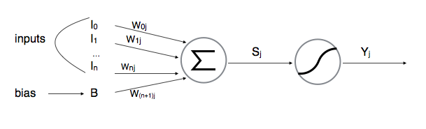
As you can see they have several inputs, for each input there's a weight (the weight of
that specific connection). When the artificial neuron activates, it computes its state
(
$$
s_j = \sum_{i} w_{ij}.y_{i} $$
where
After computing its state, the neuron passes it through its activation function
(
Activation function
The activation function is usually a sigmoid function, either a Logistic or an Hyperbolic Tangent.

Feed-forward Network
This is the simplest architecture, it consists of organizing the neurons in layers, and connecting all the neurons in one layer to all the neurons in the next one, so the output of every layer (which is the output of every neuron in that layer) becomes the input for the next layer.
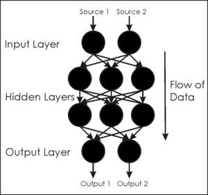
The first layer (input layer) receives its inputs from the environment, activates, and its output serves as an input for the next layer. This process is repeated until reaching the final layer (output layer).
So how does a Neural Network learn?
A neural network learns by training. The algorithm used to do this is called backpropagation. After giving the network an input, it will produce an output, the next step is to teach the network what should have been the correct output for that input (the ideal output). The network will take this ideal output and start adjusting the weights to produce a more accurate output next time, starting from the output layer and going backwards until reaching the input layer. So next time we show that same input to the network, it's going to give an output closer to that ideal one that we trained it to output. This process is repeated for many iterations until we consider the error between the ideal output and the one output by the network to be small enough.
But how does the backpropagation work?
This algorithm adjusts the weights using Gradient Descent calculation. Let's say we make a graphic of the relationship between a certain weight and the error in the network's output:
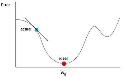
This algorithm calculates the gradient, also called the instant slope (the arrow in the image), of the actual value of the weight, and it moves it in the direction that will lead to a lower error (red dot in the image). This process is repeated for every weight in the network.
To calculate the gradient (slope) and adjust the weights we use the Delta (
Delta Rule
For the output layer (
where
The error is propagated backwards through the network until the input layer is reached.
Each layer uses the
We use the delta to calculate the gradient of each weight:
Now we can update the weight using the backpropagation algorithm:
where ε is the learning rate
Recurrent Neural Networks
Neurons in these networks have self-connections (with a fixed weight of 1) that allow them to have some sort of short-term memory.
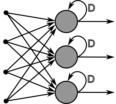
This extra input of the past activation gives the network some context information that helps it to produce a better output on certain tasks. This kind of networks prove to be very efficient in sequence prediction tasks, although they can't remember relevant information for many steps in the past.
Constant Error Carousel
The CEC consists of self-connected neuron (we'll call it memory cell), with a linear activation function. This helps the error to persist for longer time, fixing the fading gradient problem from Recurrent Neural Networks that scaled the error on each activation due to the derivation of the squashing function, making it exponentially decrease or diverge while it travels backwards through time and space. That sounds so cool.
Gates
There are architectures that not only use neurons to make connections between each other, but also to regulate the information that flows through those connections, those architectures are called second order neural networks.
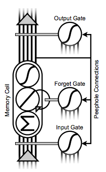
One way to protect the memory cells from noisy inputs and injected errors is to use gates to scale the connections between the memory cell and the input/output layers:
This was how the Long Short-Term Memory network architecture started. LSTM is an architecture well-suited to learn from experience to classify, process and predict time series when there are very long time lags of unknown size between important events.
Since its conception it has been improved with a third gate, called the Forget Gate, which regulates the memory cell's self-connection, deciding how much of the error should be memorized and when to forget, by scaling the feedback from the cell state after each time-step. This protects the state from diverging and collapsing.
LSTM has been also augmented with peephole connections from the memory cell to all of its gates, this improves their performance since they have information about the cell they are protecting. The actual LSTM architecture looks like this:
The math for the Recurrent and Second Order Neural Networks is a bit more complicated than the equations for the Feed-forward neural networks. I'm not going to get into that in this article, but if you are interested you should totally read Derek Monner's paper.
That's it
Now you are ready to start your journey to become a Neural Network master, you could start by checking Synaptic's demos and documentation, taking a look at the source code, or reading this paper.